Real-time bidding(RTB) refers to the buying and selling of online ad impressions through real-time auctions that occur in the time it takes a webpage to load. Those auctions are often facilitated by ad exchanges or supply side platforms(SSPs). A RTB agent has a set of active ad campaigns each with its own targeting criteria. So when an ad request is broadcasted by an ad ex or SSP, each RTB agent has to take two important decisions, first is given the segment (a segment is just the unique set of features of the incoming request e.g. geo location, content category, ad slot size, ad slot position etc) which campaign to serve from list of active campaigns and the second one is, how much to bid at.

Under The Analytical Hood.

We are starting with the assumption that given a segment S (impression request), N RTBs are actively bidding on it. We are unaware of the number N and this number is a dynamic parameter. It may happen that the campaign running on one of the competitor RTB targeting the concerned segment ends, and we are left with N-1 bidder, on the other hand new bidders can join the bidding process thereby increasing the number of active bidders.

Another interesting aspect that makes this problem more challenging is that if an RTB lost the bid, it will never get to know the auction winning price.

The number of players in the game are dynamically changing
The bid process response is either 1 (you won the bid) or 0 (you lost the bid)
At some particular bid price for a segment we have an associated win rate distribution.
The payoffs matrix is unknown i.e. we don’t know how important that segment is to the competing RTB.

We are further making an assumption that given an impression request a Pacing Algorithm has already selected a campaign and the win rate to achieve. There will be a specific win rate associated for each campaign and segment pair. Since each segment has different available inventory we can distribute our budget accordingly. So even though in next thirty minutes we are expected to receive 10000 impressions belonging to a particular customer segment we needn’t win them all. Based on all active campaigns targeting them, their respective budgets and availability of all other segments that can be targeted too our pacing algorithm outputs a win rate value. Now we will try to analytically formulate a model for the bid price prediction problem. I will try to be as much comprehensive as possible for the benefit of the uninitiated reader.

Symbols used and assumptions made :

We denote the parameters of the ith competing bidder for segment s by Bidder(i,s).
Each Bidder(i,s) is assumed to draw it’s bid price at some time ‘t’ from a Gaussian Distribution with mean=μ(i,s)t and some constant standard deviation = σ
We assume the standard deviation, σ is very small, but over time a bidder can change mean parameter of bid price.
From Game Theoretic standpoint this is a Game of incomplete information i.e. each bidder will only get to know the optimal win price only if he wins the bid and will never know what other bidders are bidding. Every player will have different set of information regarding the payoffs.
The Payoffs are continuously changing i.e. the winning rate of bids on a constant bid amount (a fixed strategy) is changing.
Each bidder i, bids on a proportion of incoming request from SSP for a particular segment s, therefore even if some bidder is bidding way less he/she will win some times since it may happen that other RTBs who usually bid higher for segment s haven’t bid on some particular requests. Lets denote the normalized bidding rate of a player i on segment s as p^i,s (Medium lacks superscript) . So we can also say that p^i,s represents the probability of bidding for an RTB i on segment s.

Since a bidder can increase or decrease its pacing rate depending time of day and remaining budget of the campaign p^i,s is a dynamic parameter.

WIN PRICE DISTRIBUTION

The Win Price distribution at time t will be a Gaussian Mixture Modelwithprobability density function(pdf) as

pdf(x) = p^1,s * N(x|mean=μ(1,s)^t , sd= σ) + p^2,s * N(x|mean=μ(2,s)^t , sd= σ) + …………………….+ p^n,s * N(x|mean=μ(n,s)^t , sd= σ)

here n refers to total number of bidder and x is the bid price.The above distribution will give us the probability density of the bid price.

So given a bid price x the above pdf will give us probability density of winning the bid.

To solve the above problem i.e. to derive the estimated values of all the distribution parameters pi,s and mean=μ(i,s)t , sd= σ we need to generate a sample (points) from the distribution and then calculate the parameters using Expectation Maximization. In the figure below the distribution is sum of two Gaussian Distribution. We can imagine that there are two bidders, each with bid price derived from one Gaussian distribution and each bids only on the proportion of requests. So the one with higher bid price always win on the bids made by it while the other won only winds a proportion of bids i.e. when the earlier bidder doesn’t bid. So the overall distribution of winning price will look like as follows

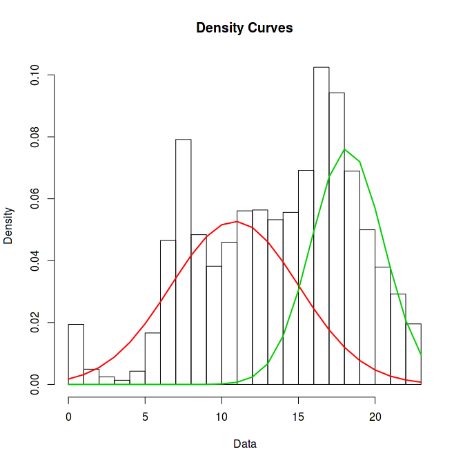
RTB1 = Green

RTB2 = Red

RTB1 has higher mean bidding price, around $18 CPM but has lower variance, whereas RTB2 has lower mean bidding price of approximately $11 CPM but has higher variance. Now given a bid price we can get an estimate of winning rate over a long run.

So sometimes RTB2 wins since it bids more than RTB1 while other times it wins because RTB1 didn’t bid on those requests.

Issues:

Now to calculate all the known parameters and draw this distribution we will need to get a sample of data points from this distribution, in our case these are the winning bid price over a significant interval of time.

In our case we never get to know the winning bid price if we lose the bid. Even if we win the bid many exchanges doesn’t reveal the second highest winning price since they don’t use Vickery auctions.
To use EM (Expectation Maximization) we should know how many RTBs are taking part in the auction, but we have on way of knowing the number ’n’ used in the pdf.
Another important issue is the temporal aspect of the distribution. It may happen that RTB1 or RTB2 stops bidding on the segment (may be their respective campaign targeting the segment finishes) or they increase the bidding rate, resulting a major change in the shape of the distribution. This kind of behavior is much expected in RTB environment.
So basically we can’t use the approach of analytically solving the Gaussian Mixture Model using Expectation Maximization.

REINFORCEMENT LEARNING : EXPLORE AND EXPLOIT

To solve the above defined mixture model we will be using a variant of a technique known as reinforcement learning that works via allocating some fixed amount of resources to exploration of the optimal solution and spends the rest of the resources on the best option. After spending due time on various explore and exploit techniques like Multi Arm Bandit,Bayesian Bandits etc I settled on using Boltzmann Exploration / Simulated Annealingtechnique.

BIDDING ALGORITHM : BAYESIAN BANDITS

We will be using Bayesian Bandit based approach using Thompson sampling for selecting optimal bandit [5]. Though bayesian bandits are mostly used in A/B testing and ad selection based on CTR, according to our research their usage suits the requirements and dynamics of RTB environment. In [6] the authors compares the performance of Bayesian Bandit techniques with other bandit algorithms like UCB, epsilon greedy etc with the aim of selecting best ad to deliver to maximize CTR. All the referred researches show that Bayesian Bandit based method outperforms other bandit techniques w.r.t. total regret, proportion of best armed played, and convergence time and readily converges to best choice/action in the explore-exploit dilemma.

Please go through the references 3, 5 and 6 for getting comprehensive look into bandit based techniques. Henceforth I will be explaining the application of Bayesian Bandit method to RTB bidding skipping the underlining theoretical details.

As described in earlier section (titled win price distribution) that the distribution of win rate and bidding price can be a mixture distribution with latent parameters. Since we will never know the winning price of a lost bid we can’t solve this optimization problem in more of an closed form analytical way. Therefore we will try to discover the optimal bid price to get the desired win rate by exploring the bid price space.

Let’s say a campaign has cpm of $5. We will divide the bid price space into different bins as follows [$1, $1.5, $2, $2.5, $3, $3.5, $4, $4.5]. Now we will explore over these bins to discover the corresponding win rate.

Experiment Scenario :

Scenario 1:

RTBS: We have 3 hypothetical RTBS bidding on a particular segment, each generating bid price via a Normal Distribution with the following bid parameters

RTB1: mean bid price = $3, standard deviation = $0.1, proportion of bids placed on incoming requests = 70% i.e. on an average this rtb bids on 70% of all requests sent by the exchange

RTB2: mean bid price = $4, standard deviation = $0.1, proportion of bids placed on incoming requests = 50%

RTB3: mean bid price = $5, standard deviation = $0.1, proportion of bids placed on incoming requests = 30%

Target Win Rate required by our test campaign = 40%

CPM = $5

Given a list of bid price choices from [$1, $1.5, $2, $2.5, $3, $3.5, $4, $4.5] bins the aim of the algorithm is to find the bin where the win rate is closest to 40%.

Examples :

Now if we bid at $3.5 cpm then the probability of winning will be = (probability that RTB3 doesn’t bid on that request) * (probability that RTB2 doesn’t bid at that request)
= (1–0.3) *(1–0.5) = 0.35
i.e. if we bid $3.5 we will win 35% of the time.
On the other hand if we bid $4 cpm then out probability of winning is = (probability that RTB3 doesn’t bid on that request) * (probability that RTB2 bid less than $4 at that request) + (probability that RTB3 doesn’t bid on that request) * (probability that RTB2 doesn’t bid at that request)
= (1–0.3) * 0.5 * 0.5 + (1–0.3) *(1–0.5)
= 0.175 + 0.35
=0.525
i.e. If we bid at $4 we will be winning 52.5% of the time.

Since the required win rate is 40% and bid price of $3.5 is giving us the win rate closest to the target win rate the algorithm should win most of the bids at $3.5

Experiment Results:

I did a simulation of the above defined scenario for 400 trials. At each request the algorithm selects a bid bin/bucket based on its assessment of win rate of that bin. Closer the win rate of the bin is to target win rate more bids will be made at that price. After each bid the algorithm will update the winning probability. After some trials the algorithm will get more and more confident about its assessment of the win rate of each bid price and will finally select the best bid price for all further bids.

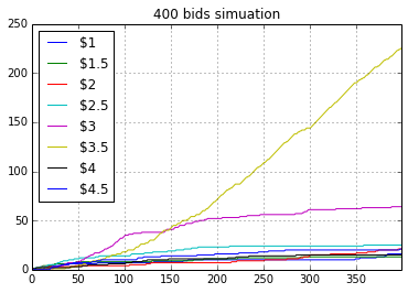
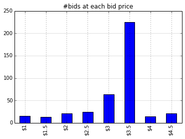
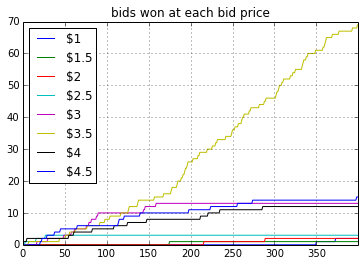
Figure 1.1 shows that for some initial runs (around 100 bids) the algorithm had enough information to make intelligent guesses about winning rate of each bid price. Once the exploration phase is over the algorithm was selecting $3.5 cpm as the bid price over and over. Figure 1.3 depicts that out of 400 bids around 225 bids were made at $3.5. The interesting aspect of the Bayesian bandit is that once the algorithm has enough confidence about the estimates of winning probability for each bid price, it was selecting $3.5 over and over (after bid #150, bid $3.5 was selected almost every time).

Issues with the Algorithm:

At each bid the algorithms updates the Posterior Distribution of the win probability of the corresponding bid price. As more and more bids take place and the algorithm’s Beta Posterior estimates converges, the variance of the posterior will be low and accurate predictions of the win rate will be made. Since the bidding environment is dynamic i.e. a new rtb can enter or an old rtb can leave the bidding process thereby changing the winning probability at some particular bid price, our algorithm will not be able to adopt to this change. The reason being that our posterior variance is too low and we have grown pretty much confident in our estimates.

Scenario 2: A new RTB enters the bidding process after 300 trials. By this time our algorithm had drawn win estimate for each bid price and has grown pretty confident about them but this new RTB will change the real win rate at $3.5 cpm bid. Now this bid will not be optimal choice for us.

RTB4: mean bid price = $3.5, standard deviation = $0.01, proportion of bids placed on incoming requests = 90%

Issues with the Algorithm:

RTB4: mean bid price = $3.5, standard deviation = $0.01, proportion of bids placed on incoming requests = 90%

Now if we bid at $3.5 our win probability will be = (1–0.3) * (1–0.5) (1- 0.9) = 0.034, i.e. 3.4%

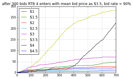
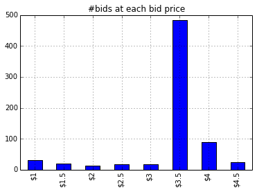
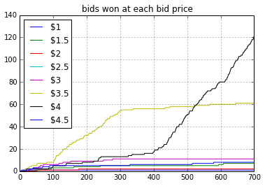
Figure 2.3 shows that as soon as RTB 4 enters the bidding process we stopped winning at $3.5 price. But since the algorithm will try to keep on believing that win rate is optimal for this bid price (think of it in terms of inertia or momentum) it will keep on bidding at $3.5. But with time it will lose the inertia and started selecting $4 cpm (after iteration 400). But overall this algorithm takes too much time to adapt to the new scenario.

RESTLESS BANDIT AND VARIANCE INFLATION

To tackle the issue of dynamic environment described in the last section, I experimented with a technique called variance inflation. As we saw in last experiment that the Bayesian Bandit technique was able to continuously pick the best bid price for an ad request just after around 100 overall bids. As we select the optimal bid price more often the variance of posterior beta will decrease. This means that our algorithm is learning continuously and becoming more and more confident about its choice. But as soon as the environment changed e.g. a new RTB bidding more than our optimal bidding price entered the bidding environment we will start losing all the bids. But it took us around 200 lost bids to learn that the current bid price is stale and that we should select some other bid price. In a way after losing hundreds of bid our algorithm lost confidence (the distribution changed) in the bid price it thought was optimal.

To tackle this problem I started increasing the variance of win rate distribution associated with each bid price by 10% as soon as we have made 50 bids on that price. This means that as soon as our algorithm starts selecting one particular bid price more often for an segment we will decrease its confidence by 10 % and ask it to explore other bid price. If the environment doesn’t change then the exploration will result in wastage of resources since we will bid either higher price or lower price then the optimal price, but if the environment changes i.e. lets say some new rtb enters or leave the bidding environment or some existing rtb starts bidding higher or lower, our algorithm will grasp this change.

Simulation Scenario:

I made the appropriate implementation changes and created similar scenario as defined in last section. We have 3 RTBs bidding for a segment with following configuration

RTB1: mean bid price = $3, standard deviation = $0.1, proportion of bids placed on incoming requests = 70% i.e. on an average this rtb bids on 70% of all requests sent by the exchange

RTB2: mean bid price = $4, standard deviation = $0.1, proportion of bids placed on incoming requests = 50%

RTB3: mean bid price = $5, standard deviation = $0.1, proportion of bids placed on incoming requests = 30%

Target Win Rate required by our test campaign = 40%

CPM = $5

Given a list of bid price choices from [$1, $1.5, $2, $2.5, $3, $3.5, $4, $4.5] bins the aim of the algorithm is to find the bin where the win rate is closest to 40%.

Objective : The bidding algorithm will find the optimal bid price i.e. $3.5 after some trials. From this point onwards our algorithm will bid on most of the requests at $3.5. But after 300 bids a new RTB, RTB 4 will enter the bidding domain. It will start bidding little more i.e. $3.6 than us. Now we will see compared to results posted in last section how fast will our new algorithm will adapt to this change and relearn the optimal bidding price.

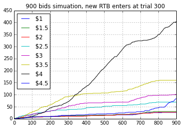
Figure 3.1 shows the over all bids made on X axis and #bids made for each bid price on Y axis. We can see that before bid #300 the optimal bid price was $3.5 and it was being used most of the time. At trial #300 a new RTB enters the bidding environment. From the above plot we can see that it took the algorithm only 20–30 trials to find that optimal bid price has changed from $3.5 to $4. Henceforth $4 bid price was selected most often.

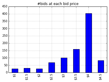
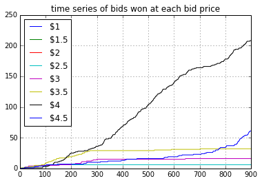
Figure 3.3 shows that the win rate for bid price $3.5 becomes nearly zero after trial #300 since RTB 4 was bidding at a higher price.

References:

IPython Notebook:
https://github.com/euclid1729/RTB_DYNAMIC_BID_PRICE?source=post_page—————————

Originally Posted by Siddharth Sharma on Medium.com, on May 10, 2016

Latest News

Contact Us

Follow Us On

Of Bandits and Bidding

WIN PRICE DISTRIBUTION

REINFORCEMENT LEARNING : EXPLORE AND EXPLOIT

BIDDING ALGORITHM : BAYESIAN BANDITS

RESTLESS BANDIT AND VARIANCE INFLATION

Resources

Company